Control System – Transient response

June 17, 2018August 5, 2019 Techie Aric 0 Comments

In my previous post , we have learnt about steady state response and steady state errors respectively. As we already know that entire time response can be split into two parts:

Transient response
Steady state response

So in this post we will learn the dynamics about ‘Transient response’ of a system. In steady state error analysis, we have seen that ‘ $e_{ss}$ ‘ was dependent on Type of the system i.e number of poles present at the origin.

Whereas, the transient response of a system depends upon the ‘Order’ of the system. Let’s understand what is ‘Order’ first.

Order of a system is the highest power of ‘s’ in the denominator of closed loop transfer function. Hence for transient response , we need to work with the ‘Closed loop transfer function’ i.e $\frac{G(s)}{1+G(s)H(s)}$ .

Analysis of ‘First Order Systems’

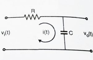
Let us take simple RC circuit, we already discussed how to find the transfer function of the below circuit

$v_i(t)$

= R i(t) + $\frac 1 {C} \int { i(t)dt }$

$v_o(t)$

= $\frac 1 {C} \int { i(t)dt }$

Now we take Laplace transform of the given system using both the above equations:

$\frac { V_{ o }(s) }{ V_{ i }(s) } =\frac { { \frac { 1 }{ sC } }I(s) }{ { R+{ \frac { 1 }{ sC } } }I(s) }$

The transfer function of the given system is

$\frac { V_{ o }(s) }{ V_{ i }(s) } = \frac{1}{sRC+1}$

This is a Closed loop transfer function, where we can see that the highest power of ‘s’ in denominator is 1. Hence RC circuit is a 1st order system since it has only one pole. The pole lies at

sRC + 1 = 0 , So, s = -1/RC

Unit Response of a 1st order system

Let us give a unit input to the R-C circuit,

hence for step input we have,

$v_i(t)$ = 1 (step input)

So, $V_i(s)$ = 1/s (taking Laplace transform both the side)

We know, $\frac { V_{ o }(s) }{ V_{ i }(s) } = \frac{1}{sRC+1}$ ,

Thus, $V_o(s) = V_i(s) .\quad \frac{1}{sRC+1}$ ,

Using partial fractions, we obtain

$V_o(s)$ = A/s + B/(s + 1/RC) ,

On Solving, we get

A = 1 , B= -1

Thus, $V_o(s) = \frac{1}{s} - \frac{1}{(s + \frac{1}{RC})}$ ,

Computing the inverse Laplace transform (knowing Laplace transforms is a prerequisite , please refer my posts on Laplace transforms) , we get

$v_o(t)$ = [1 – ${ e }^{ -t/RC }$ ] u(t)

Above is the equation for the output response, where ‘1’ is the Steady state response, and ${ e }^{ -t/RC }$ is the transient part.We can conclude that the transient part i.e ${ e }^{ -t/RC }$ is only dependent on the value of RC and not the subjected input.Hence the transient response will be same even if system was subjected to ramp or parabolic input.

Analysis of Second order System:

We considered a simple RC circuit to understand the 1st order system. We now consider RLC circuit and derive the transfer function

$v_i(t)$ = Ri(t) + Ldi(t)/dt + $\frac 1 {C} \int { i(t)dt }$

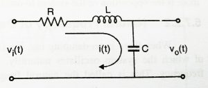
$v_o(t) = \frac 1 {C} \int { i(t)dt }$ ,

Now after taking the Laplace transform,

$\frac { V_{ o }(s) }{ V_{ i }(s) } =\frac { { \frac { 1 }{ sC } }I(s) }{ { R+ sC + { \frac { 1 }{ sC } } }I(s) }$

$\frac { V_{ o }(s) }{ V_{ i }(s) } = \frac{1}{s^2LC + sRC+1}$ (on further simplifying)

$\frac { V_{ o }(s) }{ V_{ i }(s) } = \frac{\frac{1}{LC}}{s^2 + {\frac{1}{LC}} + s\frac{R}{L}}$ ………… (2.1)

Now observe the denominator carefully, we have 2nd order equation(i.e two closed loop poles present). Now let us see more generalized , 2nd order Closed loop transfer function:

$\frac{C(s)}{R(s)} = \frac { { { \omega }_{ n } }^{ 2 } }{ s^{ 2 }\quad +\quad 2\delta \omega_{ n }s\quad +\quad { { \omega }_{ n } }^{ 2 } }$ …………….. (2.2)

We can easily compare both the above equations i.e $\omega_{ n } = \sqrt { \frac { 1 }{ LC } }$ and $\delta = \frac{R}{2}\sqrt { \frac { C }{ L } }$ for a RLC circuit. Equation (2.2) represents the standard second order transfer function. In the equation, ‘ $\omega_{ n }$ ‘is called the natural frequency while ‘ $\delta$ ‘ (zeta) is called the Damping factor.

We should now look into the significance of these two terms. Damping Factor and Natural Frequency of Oscillation can be explained as below:

Damping Ratio (‘ $\delta$ ‘) :

Generally system takes some time to achieve the ‘Steady state value’ , During this time the system either oscillates or increases exponentially.

Every system has a tendency to oppose any oscillatory behaviour.This opposition to oscillation is called damping. Damping is measured by a factor called the damping ratio. Higher the damping ratio more is the opposition to oscillation.

Natural Frequency of Oscillation (‘ $\omega_{ n }$ ‘) :

When the damping ratio is ‘0’ i.e there is no opposition present for the oscillatory behaviour, system will oscillates with maximum frequency.

This frequency is called as ‘Natural Frequency of Oscillation’. For eg in the RLC circuit we discussed, its damping $\delta = \frac{R}{2}\sqrt { \frac { L }{ C } }$ , will be zero and the RLC circuit will oscillate with a natural frequency given by the formula $\omega_{ n } = \sqrt { \frac { 1 }{ LC } }$

Position of Poles in a 2nd order System

We have seen that in a 1st order system, it has only one closed loop pole. If we change any system parameter, it will surely change entire form of the response. A single pole can move only on the real axis and hence for any 1st order system we have purely exponential response. Now compared to first order system, second order system exhibits a wide range of responses. These two closed loop poles can move anywhere in the s-plane when system parameters are changed.

Effect of ‘ $\delta$ ‘ on the position of Closed loop poles:

The standard second order transfer function is given by:

$\frac{C(s)}{R(s)} = \frac { { { \omega }_{ n } }^{ 2 } }{ s^{ 2 }\quad +\quad 2\delta \omega_{ n }s\quad +\quad { { \omega }_{ n } }^{ 2 } }$

The Closed loop poles are

${ s^{ 2 }\quad +\quad 2\delta \omega _{ n }s\quad +\quad { { \omega }_{ n } }^{ 2 } }$ = 0 ,

$s_{ 1,2 }=-\delta { \omega }_{ n }\quad \pm \quad { \omega } _{ n }\sqrt { { \delta }^{ 2 } -1 }$

For a given system value of ‘ $\omega }_{ n }$ ‘ will be constant. Hence the position of poles depend on the value of ‘ $\delta$ ‘

We now consider 4 cases

When 1 < $\delta$ < infinity (assume any values in the values of the two roots above)

It can be observed that the poles are real , unequal and negative

When $\delta$ = 1 (put value of $\delta$ as 1 in the value of roots),

In this case both the poles are at $-\omega_n$ i.e there is double pole at s = $-\omega_n$

When 0 < $\delta$ < 1

It can be seen that the poles are complex conjugate of each other.

when $\delta$ = 0

$s_1$ = j $\omega_n$ $s_2$ = -j $\omega_n$

The poles have no real part and lie on the imaginary axis.

Now we shall see the type of system based on the values of the ‘ $\delta$ ‘(refer diagram):

Undamped( $\delta$ = 0)
Underdamped( $\delta$ < 1)
Critically damped( $\delta$ = 1)
Overdamped ( $\delta$ > 1)

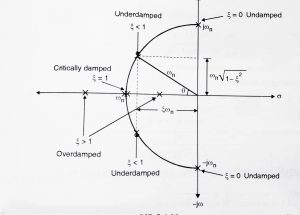
In the above figure damping ratio ( $\delta$ ) has been represented as $\xi$ .From the above diagram, you can get the location of the closed loop poles for different values of damping ratio.

Techie Aric

Aric is a tech enthusiast , who love to write about the tech related products and ‘How To’ blogs . IT Engineer by profession , right now working in the Automation field in a Software product company . The other hobbies includes singing , trekking and writing blogs .

Spread the Wisdom !!

Techie Aric

You May Also Like

Leave a Reply Cancel reply