Control System – Root Locus (Some Additional Points) !!

If you have already gone through my earlier posts, you shall already be knowing by now the exact meaning of roots and characteristic equations of CLTF. So for a quick recap, the roots associated with any characteristic equation of system are the poles associated with the system, they further combined with the zeros will determine the response of this system.

The branches associated with root locus tells you how the located area of the poles change when you raise (increase) the gain for the given system (k) . While plotting on the main locus, we plot the roots of this characteristic equation as part of the gain and not frequency. So It isn’t a frequency-domain system.

Now we may further see some additional important points regarding Root locus method:

1.If there are more zero and fewer poles

If the number of zeros is greater,  then the number of loci = z.

Number of loci ending at ∞ equals z – p . All other rules remain same.

2.Value of Gain Margin:

Gain Margin for Root Locus is given as

Gain Margin =

When the root locus does not cross j  axis then gain is ∞.

Gain margin indicates the highest gain that can be multiplied to the system in order to just make it on the edge (verge) of instability.

3.Phase Margin from Root Locus :

For a given value of k, the phase margin can be given as:

• Find out  by |GH(j)| =  1  for design value of k.
• Find arg GH ( j )
• Phase margin = 180 + arg GH(j)

Effect of Addition of poles and Zeros on root Locus:

1.Effect of Addition of poles :

The basic effect of the inclusion of a pole is the tendency to shift the complete root locus towards the right half of s-plane . This lowers the stability. Let’s consider a system :

G(s)H(s) =   , its root locus is shown below:

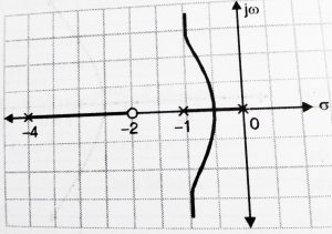
Now , consider system  G(s)H(s) =    , in this root locus  is shown below:

 

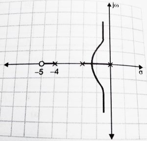
Now, let’s add a pole at s = -1.5,

G(s)H(s) =     , it’s root locus is shown below:

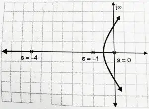
Thus the system will become unstable at some value of k.

If instead of  -1.5 , pole was added at s = -5 , the system would eventually become unstable, but the crossover would take place at a much higher value  of k.

The addition of pole brought the closed-loop poles towards the j  axis making the system more oscillatory. Among the poles s = -2 and -1.5 , s= -1.5 affects the change more on account of its nearness to j  axis and origin. Hence it is referred  as dominant pole.

2.Effect of addition of zeros:

The general effect of the addition of zero is a tendency to pull the root locus to the left half of s-plane . Hence adding zeros increase stability.

Consider,         G(s) H(s) =    ,  it’s root locus is given by:

 

Now if we add a zero at  s = -5 , the root locus is given by

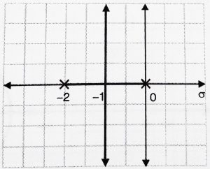
Now, if we add progressively dominant pole i.e s = -2 and not s = -5, we get the root locus as:

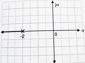
We can see that the system becomes more stable.

The addition of zeros thus speeds up settling time (as it pulls the locus to the left) and stabilizes the system.

Lastly, you should realize that this method is used in order to find the values of  ‘k’ (i.e. system gain) for which a given closed-loop system will be stable.

The crux (central point) here is that if we in case further add any additional controller (or if we modify the system gain) to our process , then we can adjust the system so as to meet our specific requirements.

For e.g. if a required motor is not moving fast enough, then we have to add a controller which will simply increase the current or voltage to the motor (and thus the motor rotates faster).

So this is it for time response analysis(hope you really enjoyed),  from my next post onwards we will be looking into frequency response analysis of a system.