Control System – Steady State Response
As already discussed in my previous post, in this part(steady state) the output response will remain constant. The parameter which will be our main focus is the ‘Steady state error’(remember the elevator example I depicted in my previous post, the lift stopped at 10.5 and not 11).So for reference we will again refer the complete time response of a system,
Error in general is nothing but the difference between input(desired) and output(actual).It is given as error at ![]() ,
,
![]()

R(s) = Laplace of input R(t)
C(s) = Laplace of output
B(s) = Laplace of feedback signal
E(s) = Laplace of error signal
G(s) = Transfer function of main system
H(s) = Transfer function of feedback element
E(s) = R(s) – B(s), But B(s) = C(s) . H(s)
E(s) = R(s) – C(s).H(s) Also, C(s) = E(s).G(s)
E(S) = R(s) – E(s) G(s) H(s)
Hence the equation for generalized error in Laplace domain is:
![]()
But we want error occurring after very long time i.e at ![]() , so we now use the final value theorem in the Laplace domain ,
, so we now use the final value theorem in the Laplace domain ,
i.e ![]()
On applying Final Value theorem , we get
![]() ,
,
![]() ………… (1.1)
………… (1.1)
From above equation , we can note that ![]() depends on two factors:
depends on two factors:
- Input R(s)
- Open loop transfer function G(s).H(s)
We shall discuss these two factors in detail now:
- Effect of input R(s)
We have already seen the standard test inputs(in my previous post) , We will now see effect of step, ramp and parabolic inputs on the steady state error.
Static Error Coefficient:
The difference between the steady state response and desired response gives us steady state error. A Control System has the following steady state error constants for changes in position, velocity and acceleration:
 = Positional error constant
 = Velocity error constant
 = Acceleration error constant
These error constants are called as ‘Static error coefficients’ . They have the ability to minimize the steady state error. Now let us analyse the individual inputs :
- Step Input
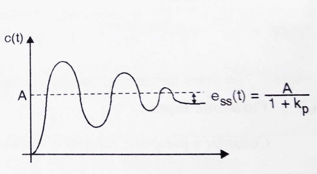
Consider a step input of magnitude ‘A’ is applied as reference input to the system.We already know in Laplace domain it will be given as
![]() ,
,
Using equation (1.1) we have,
![]() ,
,
Now, ![]() ,
,
Then , ![]() …………………..(1.2)
…………………..(1.2)
Now let us introduce the positional error coefficient, it is denoted by ‘ ![]() ’ and defined as
’ and defined as
![]() ,
,
Putting this value in equation (1.2),
![]() ,
,
Above equation indicates that, when a step input is subjected to a system, the steady state error is controlled by positional error coefficient .

- Ramp input
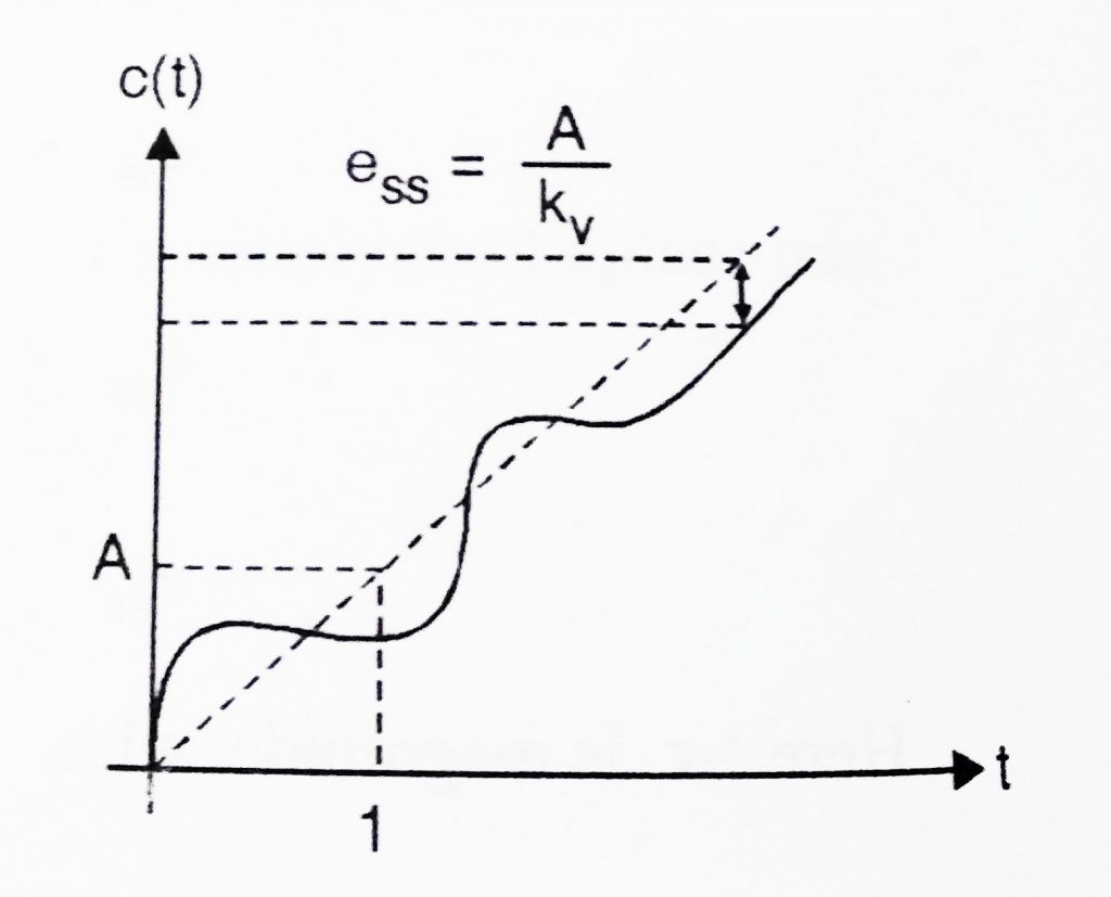
Consider a Ramp input of magnitude ‘A’ , which is applied as reference input to a system. We already know, this input can be represented in Laplace domain as:
![]() ,
,
Using equation (1.1),we have
![]() ,
,
![]() ,
,
Also we know,
![]() ,
,
Hence, ![]() ……… (1.3)
……… (1.3)
Now let us introduce the velocity error coefficient, it is denoted by ‘ ![]() ’ and defined as
’ and defined as
![]() ,
,
Putting this value in equation (1.3),
![]() ,
,
Above equation indicates that, when a Ramp input is subjected to a system , the steady state error is controlled by velocity error coefficient .

- Parabolic Input
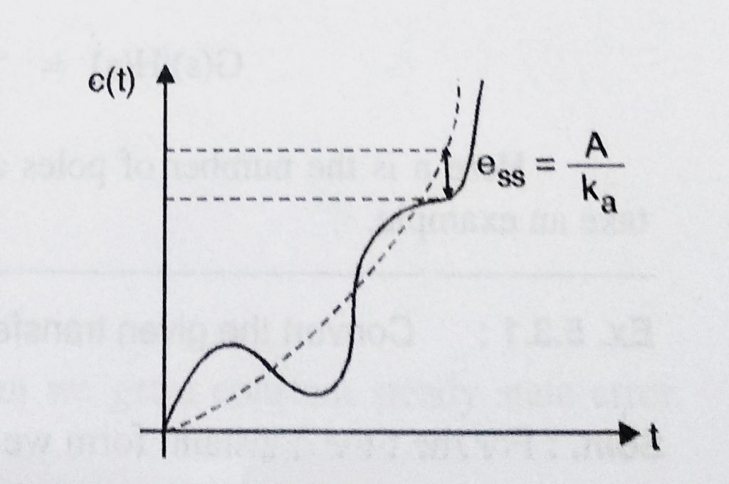
Consider a parabolic input of slope ‘A/2’ , which is applied as reference input to a system. We already know this input can be represented in Laplace domain as:
![]() ,
,
Using equation (1.1), we have
![]() ,
,
![]()
Also we know,
![]() ,
,
Hence, ![]() ……… (1.4)
……… (1.4)
Now let us introduce the acceleration error coefficient, it is denoted by ‘ ![]() ’ and defined as
’ and defined as
![]() ,
,
Now , Putting this value in equation (1.4),
![]() ,
,
Above equation indicates that, when a parabolic input is subjected to a system , the steady state error is controlled by velocity error coefficient .

Quick recap of steady state errors with different error coefficients :
 …………………. For step input
 …………………. For Ramp input
 ………………… For parabolic input
Now we shall see effect of Open Loop Transfer function G(s).H(s) on steady state error ![]() :
:
Actually it depends upon the ‘Type’ of the system G(s)H(s). Let us define what we mean by type of a system now,
A ‘Type’ of any control system is basically defined in terms of the total number of the open loop poles i.e the poles of G(s)H(s) that lies at the origin.
Hence ![]() is a ‘type 0’ system as no poles present at the origin.
is a ‘type 0’ system as no poles present at the origin.
Similarly ![]() and
and ![]() are type 1 and type 2 systems respectively.
are type 1 and type 2 systems respectively.
In the next post we will see the effects of subjecting standard test inputs to various ‘Types’ of systems.

Aric is a tech enthusiast , who love to write about the tech related products and ‘How To’ blogs . IT Engineer by profession , right now working in the Automation field in a Software product company . The other hobbies includes singing , trekking and writing blogs .
