Control System – Time Response Analysis

In this post, we will look into the various characteristics of the response in any control system. Time response analysis means subjecting Control system to inputs that are functions of time and analyzing their outputs which are also functions of time.

So before we dig deep inside this concept, let’s understand this topic in layman’s term (by relating this to daily life example).

Consider an example of an elevator. When we press 11^th floor button in the lift, the motor of the elevator starts moving. Considering passenger’s safety, the elevator will not suddenly shoot off to 11^th floor. Instead, it will reach in smooth manner.Also  we want it to reach the desired floor and not get stuck between two floor(the concept of steady-state error discussed later).

Having a clear picture of desired and specific requirements, we can now list down the elevator time response against the input (of pressing 11th-floor button in the lift):

Refer below figures for the time response of the elevator

In fig ‘a’, output rises gradually. The elevator is extremely slow. Elevator stops between  10^th and   11^th floor.

In fig ‘b’ , response of elevator is faster than fig ‘ a’ , but the elevator still stops between 10^th and 11^th

In fig ‘c’ response is very fast, and it initially oscillates between 10^th and 12^th floor before settling down on the 11^th floor

In fig ‘d’ we have the best time response. The elevator rises in a smooth manner and stops exactly at the 11^th

Let’s now look at the complete time response of the above scenario and further define some important terms present:

fig (a)                                                                                                                fig (b)

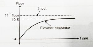
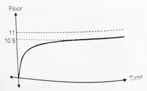
Fig (c)                                                                                                                               fig (d)

 

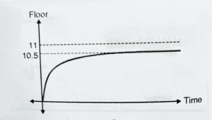
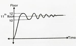
The entire time response is divided into two parts(1  and 2) . In part 1, the output is changing with respect to time(gradually) and in part 2 , the output is almost constant.

Part 1 is called transient response while part 2 is called ‘steady state response’. Hence transient time response is the part where the response is changing with respect to time, while steady-state response is that part where time response of output is more or less constant.

 

 

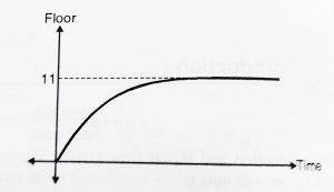
We note that output settles down  at 10.5 instead of 11 , this error is known as steady-state error and is associated with steady-state response. The transient response may be exponential or oscillatory.

Total time response ,c(t) is the transient response

(t) followed by the steady state response  (t).

c(t) = transient response + steady-state response

c(t) =  (t) +  (t)

Now we should learn some of the known input signals. For analyzing the response we need to subject the system to various test inputs. So some of the standard test signals that are used are:

• Impulse    
• Step
• Ramp
• Parabola
• Sinusoid

Now we shall look in brief about these input signals:

Impulse input:

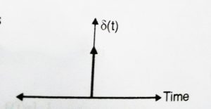
As the name indicates, it represents a sudden change in the input. An Impulse signal is infinite at t = 0 and zero anywhere else. Thus the area enclosed by the curve is 1. It further has  a magnitude of ‘1’ at time t = 0.

R(t) = 1     at  t = 0,

R(t) = 0     at   t   0,

 

In Laplace domain this can be given as R(s) = 1

Step input:

The input given to the elevator is a Step input. It represents constant command such as position. It can be given as:

R(t) = A      at t  0 ,

R(t)  =  0     otherwise,

In case of unit step, we will have R(t) = 1;

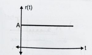
In Laplace domain this can be given as R(s) =

Ramp input:

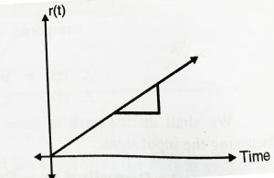
It indicates linear increasing nature ( y = mx nature). It is given as

R(t) = At             t  0 ( ‘A’ is the slope)

R(t) = 0                    t 0,

In Laplace domain this can be given as R(s) =

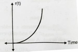
Parabolic input :

The Rate of change of velocity is acceleration. Acceleration is parabolic in nature. This input is given as:

R(t) = (A/2)       t 0 ;

R(t) =   0               t 0 ;

In Laplace domain this can be given as R(s) =  

Sinusoidal input:

This signal is used to study the frequency responses. We need to subject input of varying frequency to a system, in order to study the frequency response. It is given as:

R(t) = A sin(ωt) ,

 

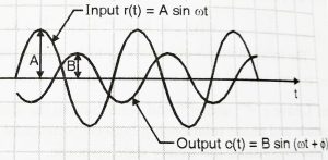
For time response analysis we will not consider this input (this will be considered for frequency response analysis).

We shall now discuss the two parts of time response (transient and steady-state as discussed earlier) in our next post.We will see steady-state response first as it is easier and then follow it up by transient response.