Control System – Subjecting a Type 0, Type1 and Type 2 system to Test Inputs

June 17, 2018August 5, 2019 Techie Aric 0 Comments

As we already seen in the last post about the ‘steady state error’ associated with ‘steady state’ response of any control system. Now we shall see different ‘Types'(depending upon number of poles present at the origin) of system and their behavior when subjected to different test inputs. So without wasting much time, let’s start the analysis.

A ‘Type 0’ system is given by

$G(s)H(s)=\quad \frac { k(1+T_{ z1 }s)(1+T_{ z2 }s)……… }{ s^{ 0 }(1+T_{ p1 }s)(1+T_{ p2 }s)…….... }$ (no pole at origin)

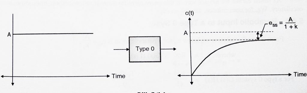
1.1 Step input to a Type 0 system:

From my previous post , we already know the steady state error ‘ $e_{ss}$ ‘ for a step input is

$e_{ss}= \frac A {1 + k_p}$ ,

where $k_p = \underset { s\to 0 }{ \lim }{G(s)H(s)} = \underset { s\to 0 }{ \lim } \frac { k(1+T_{ z1 }s)(1+T_{ z2 }s)……… }{ s^{ 0 }(1+T_{ p1 }s)(1+T_{ p2 }s)…….... }$

$k_p = \frac{k(1)(1)....}{s^0(1)(1)....}$

= k ,

$e_{ ss }=\frac { A }{ 1+k_{ p } } =\frac { A }{ 1+k }$ ,

Hence when a type 0 system is subjected to a step input, we get a constant steady state error.

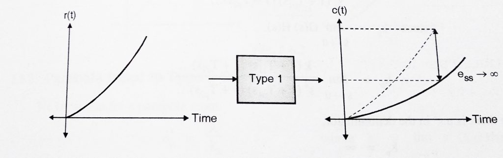
1.2 Ramp input to a Type 0 system:

From my previous post , we already know the steady state error ‘ $e_{ss}$ ‘ for a ramp input is

$e_{ss}= \frac A { k_v}$

where $k_v = \underset { s\to 0 }{ \lim }{sG(s)H(s)} = \underset { s\to 0 }{ \lim } \frac { sk(1+T_{ z1 }s)(1+T_{ z2 }s)……… }{ s^{ 0 }(1+T_{ p1 }s)(1+T_{ p2 }s)…….... }$ = 0,

$k_v= \frac{sk(1)(1)....}{s^0(1)(1)....}$ = 0 ,

$e_{ss}= \frac{A}{k_v} = \frac{A}{k}$ = ∞(infinity) ,

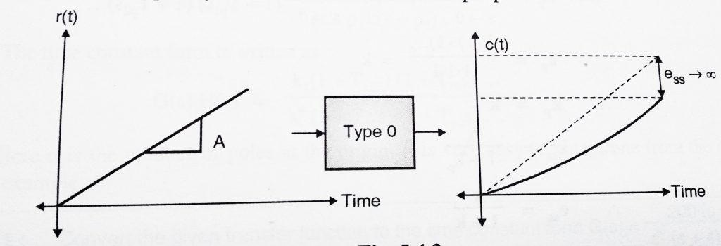
Hence when we subject a type 0 system to a ramp input, the steady state error increases continuously.

1.3 Parabolic input to a Type 0 system:

From my previous post , we already know ‘ $e_{ss}$ ‘ for a parabolic input is

$e_{ss}= \frac A { k_a}$ where $k_a = \underset { s\to 0 }{ \lim }{{s^2}G(s)H(s)} = \underset { s\to 0 }{ \lim } \frac { {s^2}k(1+T_{ z1 }s)(1+T_{ z2 }s)……… }{ s^{ 0 }(1+T_{ p1 }s)(1+T_{ p2 }s)…….... }$ = 0,

$k_a= \frac{s^2k(1)(1)....}{s^0(1)(1)....}$ = 0 ,

$e_{ss}= \frac{A}{k_a} = \frac{A}{k}$ = ∞(infinity) ,

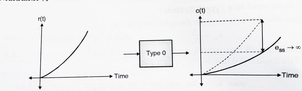
Hence when we subject a type 0 system to a parabolic input, the steady state error increases continuously. Hence type 0 system are not suitable when the input is parabolic in nature.

Now we shall shift our focus to type 1 systems:

A ‘Type 1’ system is given by

$G(s) H(s) = \underset { s\to 0 }{ \lim } \frac { k(1+T_{ z1 }s)(1+T_{ z2 }s)……… }{ s^{ 1 }(1+T_{ p1 }s)(1+T_{ p2 }s)…….... }$ = 0 (one pole at origin)

2.1 Step Input to Type 1 System:

we already know ‘ $e_{ss}$ ‘ for a step input is

$e_{ss}= \frac A { 1+k_p}$ where $k_p = \underset { s\to 0 }{ \lim }{G(s)H(s)} = \underset { s\to 0 }{ \lim } \frac { k(1+T_{ z1 }s)(1+T_{ z2 }s)……… }{ s^{ 1 }(1+T_{ p1 }s)(1+T_{ p2 }s)…….... }$ ,

$k_p= \frac{k(1)(1)....}{s^1(1)(1)....}$ = ∞ (infinity) ,

$e_{ss}= \frac{A}{1+k_p} = \frac{A}{1+k}$ = 0 ,

Hence when a type 1 system is subjected to a step input, we get steady state error i.e . $e_{ss}= 0$ . Hence we can conclude that type 1 systems are excellent for step inputs as steady state error is 0.

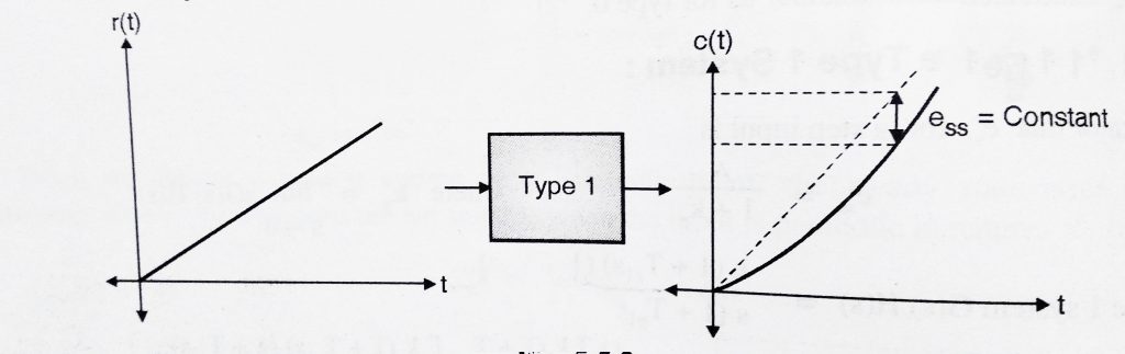
2.2 Ramp input to a Type 1 System

we already know ‘ $e_{ss}$ ‘ for a ramp input is

$e_{ss}= \frac A { k_v}$

where $k_v = \underset { s\to 0 }{ \lim }{sG(s)H(s)} = \underset { s\to 0 }{ \lim } \frac { sk(1+T_{ z1 }s)(1+T_{ z2 }s)……… }{ s^{ 1 }(1+T_{ p1 }s)(1+T_{ p2 }s)…….... }$ ,

$k_v= \frac{sk(1)(1)....}{{s^1}(1)(1)....}$ = k ,

$e_{ss}= \frac{A}{k_v} = \frac{A}{k}$ = constant ,

Hence when we subject a type 1 system to a ramp input, the steady state error is constant.

2.3 Parabolic Input to a Type 1 System:

we already know ‘ $e_{ss}$ ‘ for a parabolic input is

$e_{ss}= \frac A { k_a}$ where $k_a = \underset { s\to 0 }{ \lim }{{s^2}G(s)H(s)} = \underset { s\to 0 }{ \lim } \frac { {s^2}k(1+T_{ z1 }s)(1+T_{ z2 }s)……… }{ s^{ 1 }(1+T_{ p1 }s)(1+T_{ p2 }s)…….... } = 0$ ,

$k_a= \frac{s^2k(1)(1)....}{s^1(1)(1)....} = 0$ ,

$e_{ss}= \frac{A}{k_a} = \frac{A}{k}$ = ∞(infinity) ,

Hence when we subject a type 1 system to a parabolic input, the steady state error increases continuously. Hence type 1 system are not suitable when the input is parabolic in nature.

Let’s now proceed further and analyze type 2 systems:

A ‘Type 2’ system is given by

$G(s) H(s) = \underset { s\to 0 }{ \lim } \frac { k(1+T_{ z1 }s)(1+T_{ z2 }s)……… }{ s^{ 2 }(1+T_{ p1 }s)(1+T_{ p2 }s)…….... }$ = 0 (two poles at origin)

3.1 Step Input to a type 2 System

we already know ‘ $e_{ss}$ ‘ for a step input is

$e_{ss}= \frac A { 1+k_p}$ where $k_p = \underset { s\to 0 }{ \lim }{{G(s)H(s)} = \underset { s\to 0 }{ \lim } \frac { k(1+T_{ z1 }s)(1+T_{ z2 }s)……… }{ s^{ 2 }(1+T_{ p1 }s)(1+T_{ p2 }s)…….... } = 0$ ,

$k_p= \frac{k(1)(1)....}{{s^2}(1)(1)....}$ = ∞ (infinity) ,

$e_{ss}= \frac{A}{1+k_p} = \frac{A}{1+k} = 0$ ,

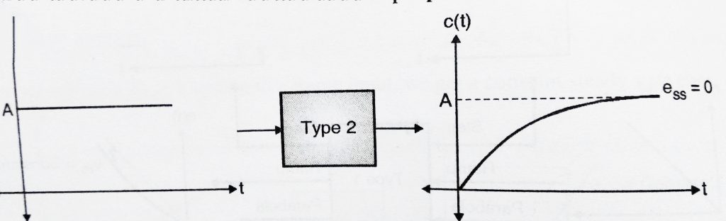
Hence when a type 2 system is subjected to a step input, we get steady state error i.e . $e_{ss}$ = 0. Hence we can conclude that type 2 systems are excellent for step inputs as steady state error is 0.

3.2 Ramp input to a Type 2 System

we already know ‘ $e_{ss}$ ‘ for a ramp input is

$e_{ss}= \frac A { k_v}$ where ,

$k_v = \underset { s\to 0 }{ \lim }{sG(s)H(s)} = \underset { s\to 0 }{ \lim } \frac { sk(1+T_{ z1 }s)(1+T_{ z2 }s)……… }{ s^{ 2 }(1+T_{ p1 }s)(1+T_{ p2 }s)…….... }$

$k_v= \frac{sk(1)(1)....}{{s^2}(1)(1)....}$ = ∞ ,

$e_{ss}= \frac{A}{k_v} = \frac{A}{k}$ = 0 ,

Hence when we subject a type 2 system to a ramp input, the steady state error is 0.

3.3 Parabolic Input to a Type 2 System:

we already know ‘ $e_{ss}$ ‘ for a parabolic input is

$e_{ss}= \frac A { k_a}$ where ,

$k_{ a }=\underset { s\to 0 }{ \lim } { ({ s^{ 2 } }G(s)H(s) }=\underset { s\to 0 }{ \lim } \frac { s^{ 2 }k(1+T_{ z1 }s)(1+T_{ z2 }s)……… }{ s^{ 2 }(1+T_{ p1 }s)(1+T_{ p2 }s)…….... }$

$k_{ a }=\frac { { s^{ 2 } }k(1)(1).... }{ { s^{ 2 } }(1)(1).... }$ = k ,

$e_{ss}= \frac{A}{k_a} = \frac{A}{k}$ = const ,

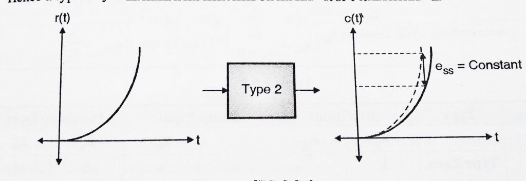
Hence when we subject a type 2 system to a parabolic input, the steady state error is constant. Hence we can conclude that Type 2 systems are excellent for step and ramp signals and gives constant error for parabolic inputs.

For quick summary of this post you may refer below table:

Sr no	Type	Step input		Ramp input		Parabolic Input
		$k_p$	$e_{ss}$	$k_v$	$e_{ss}$	$k_a$	$e_{ss}$
1	Type 0	k	$\frac A {1+k}$	0	∞	0	∞
2	Type 1	∞	0	k	$\frac A {k}$	0	∞
3	Type 2	∞	0	∞	0	k	$\frac A {k}$

Before ending this post, I like to add few disadvantages of static error coefficient method:

They can be used only for three standard test inputs.(i.e they cannot give error for inputs other than these)
Only extreme values of error i.e 0 and ∞ (infinity) are specified. The exact value of error not specified.
This method doesn’t provide information about error variation with time.
It is only applicable to stable system and not to unstable system.

These drawbacks can be overcome by using ‘Dynamic error coefficients (also called as generalised error coefficient).

Hope you really enjoyed this post, meet you soon in my next post.

Techie Aric

Aric is a tech enthusiast , who love to write about the tech related products and ‘How To’ blogs . IT Engineer by profession , right now working in the Automation field in a Software product company . The other hobbies includes singing , trekking and writing blogs .

Spread the Wisdom !!

Techie Aric

You May Also Like

Leave a Reply Cancel reply