Control System – Signal Flow Graphs

Signal flow graph is an alternative to Block Reduction technique. Here instead of blocks, take-off points, summing points etc , we have to deal with branches and nodes.

Significance of Signal flow graph over Block reduction technique

Both the method will help us to find the overall transfer function of the system. In case of Block reduction technique, we need to analyze the whole system in simplified small parts. In the case of complex system, finding the overall transfer function will become very much tedious.

Signal flow graph on the other hand uses single formula known as ‘ Mason’s Gain Formula’ to achieve the same result(and hence takes less time and efforts).

Let us first understand how to draw a signal flow graph from the equation and then use them for the control system. Every control system consists of nodes (dependent and independent variables).

These nodes are connected together by a line called as ‘ Branches’.Consider simple equation           

     

 

 

 

Here and 

   are called ‘Nodes’ and ‘A’ is the gain. The arrow indicates the direction of the signal flow.

Let’s take an example to make this topic clear

Consider a system represented by the following equations,

       ;               

  ;

    ;                    ;

We shall draw  SFG for individual equation first and then draw the combined SFG

1.    

 

2.  

 

 

3.  

 

4.  

Now on combining all the above figures,we can obtain the following signal flow graph(consisting of 5 variables ):

 

Method to draw Signal flow graph that can be deduced from any Block Diagrams

We shall now see how to draw Signal flow graph from Block Diagrams, for this we have to follow below-mentioned steps:

• Represent each summing point and take-off point as a separate node.
• Connect each of them by branches
• The block transfer function is represented as branch gain
• Show input and output nodes separately with branch gain as 1

 

Let us take one example to make this more clear

We will now represent a block diagram as a signal flow graph:

 

We can identify the nodes of the SFG  by marking the summing points and the take off points.

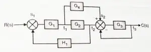
Finally the signal flow graph can be shown as:

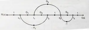
As we can see from above, we can easily deduce signal flow graphs from complex block diagrams. Finally we required to learn some methods in order to reduce any signal flow graph consisting of any number of branches and nodes.

Some important Signal Flow Graph Terms

Now we will learn some common terms that we may encounter while reducing any system by the Signal Flow Graph   method .  

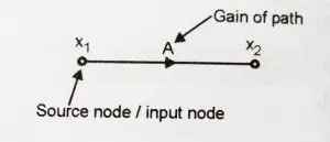
1. Source or Input node

A source node can be defined as the node that has just the outgoing branches from it. 

 

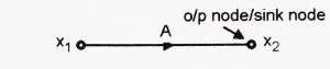
2. Output or Sink node

This node has only incoming branches.

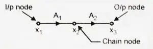
3. Chain node

This node will have both incoming and outgoing branches

 

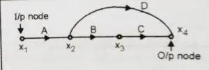
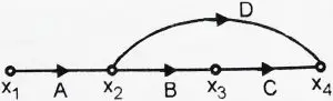
4. Forward path

This is a path from input to output node is a forward path

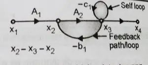
5. Feedback path (or feedback loops)

A path which originates and terminates on the same point (node).

This can be called as ‘Self loop’ when it consist of only one node in Self loop

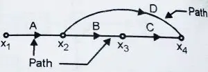
6. Path gain

The product of all the branch gains while going through a forward path is called the path gain. Here the path                    gain  for the path x1-x2-x3-x4 is A x B x C.

7. Path

This can be found out by seeing the connected branches, any path will be along the way of the signal  flow , and no node is traversed more than once.

 

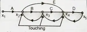
8. Touching Path

A loop and Path when have a node in common, then they are said to be touching. Also if there are one or more common nodes in any loops, then they are said to be touching loops.

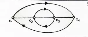
9. Non Touching Loops

If there are no common nodes present between any loops, then they are known as the non touching loops.

 

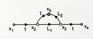
10. Loop gain

It is simply the product of every branch gains forming a loop is called as loop gain. For the path x2-x3-x5-x2 the loop gain is                 L1  x L2 .

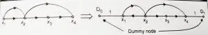
11. Dummy nodes

A branch having gain of ‘1’ can be added at input as well as output. They cannot be added in between the chain nodes. This addition will not affect the transfer function in any manner.

Properties of SFG (Signal flow graph)

Every block diagram can be represented by SFG but the converse is not true.

 

It applies only to time-invariant linear system.

 

The value of the variable at each node is equal to the algebraic sum of all signals entering at that node.

 

The gain of SFG is given by Mason’s equation.

 

In the next post , we will see how to implement these rules to reduce any given complex block diagram system using the signal flow graph technique(by taking the help of Mason’s equation).