Control System – Block Diagram Reduction Rules !!

Spoiler : This post is long yet interesting!!

As we already know that control systems consist of mathematical models. The transfer function is a mathematical representation of the individual physical system. To show the function performed by each component, we generally use a  block diagram.

Thus in order to analyze complex control systems (and hence complex block diagrams), it is much desirable to reduce the block diagram in simple terms(by means of block diagram reduction techniques).

Thus in simple terms, a block diagram is a pictorial representation of the entire system. In this manner, it represents the relationship between input and the output of entire system.

Block diagram definitions:

1. Block diagram: This gives a pictorial relationship between output and input of the system.

2. Output: It is defined as product of input and gain i.e    Output = gain x input

3. Summing point: A point where multiple signals can be subtracted or added respectively.

4. Take off point: From this point, the output can be again fed back to input, thus this point will be used for feedback purpose.

5. Forward path: This path represents the direction of the signal flow in the system from the input side to output side.

6. Feedback path: This path represent direction of the signal flow in the system from output side to input side.

 

The first step will be to obtain the block diagram from a physical system(can consist of anything like amplifier, potentiometer etc).

Once the block diagram is obtained, now we need to obtain the transfer function. For analyzing, we have to simplify the (complex) block diagram into one single block.

This way of reducing a complex block diagram into a single block representing the transfer function of the entire control process is called as the ‘Block Diagram Reduction’ technique.

Basic Closed loop Transfer Function (most important formula) !!

Before we proceed to find the transfer function of complex block diagrams, we should first check out the basic closed-loop transfer function,

Consider a simple closed-loop system,

R(s) = Laplace of input signal

C(s) = Laplace of output signal

E(s) = Laplace of error signal

B(s) = Laplace of feedback signal

G(s) =  forward transfer function

H(s) = feedback transfer function

 

If negative feedback is present in the system,

If positive feedback is present in the system,

   

 

Also for open-loop transfer function, as no feedback present, transfer function can be given by:

Open loop transfer function = G(s).H(s)

Block Diagram Reduction Rules

We need to follow certain rules to reduce any given complex control system into a simpler form. So following are the most widely used block diagram reduction rules(each one will be discussed in detail)

• Rule 1: Blocks in cascade/series
• Rule 2: Blocks in parallel
• Rule 3: Feedback loop elimination
• Rule 4: Associative law for summing
• Rule 5: Shifting a summing point before a block
• Rule 6: Shifting a summing point after a block
• Rule 7: Shifting take-off point before a block
• Rule 8: Shifting take-off point after a block
• Rule 9: Shifting a summing point before a block
• Rule 10: Shifting a summing point after a block

For simplicity, we will write G(s) as ‘G’ and H(s) as ‘H’ . Now in the next section, we will explore each of the above rules in detail and precisely understand its application. 

Shortcut Rules For Reducing Any Complex Block Arrangement !!

Rule 1: Blocks In Series

Any finite specific number of blocks arranged in series can be combined together by multiplication as shown below:

The above blocks shown can be combined together and replaced with single block as

Output C(s) = G1 x G2 x R(s)

If there is a take-off point or summing point between the blocks, the blocks cannot be said to be in cascade/series.(the take-off/summing point has to be shifted before or after the block using another rule)

Rule 2: Blocks In Parallel

When the blocks are connected in parallel combination, they get added algebraically (considering the sign of the signal)

 

this can be combined as(refer both the diagrams)

 

The above blocks can be replaced with a single block as

C(s) = R(s)G1 + R(s)G2 – R(s)G3

C(s) = R(s) (G1 + G2 – G3)

If any summing point/take-off point is present in between the blocks, then that has to be shifted first.(in a parallel arrangement, the direction of signal flow must be in the same direction through all the blocks)

Rule 3: Elimination of  feedback Loop

We can use Closed loop transfer function to eliminate the feedback loop present.(Always remember for applying this method the direction of  flow of signals should be in opposite direction, otherwise, if they are in the same direction, then we need to apply parallel reduction technique discussed above)

   

Now consider the application of the above three rules together and refer to the block diagram above.

Rule 4: Associative Law For Summing Point

This can be better explained by taking below diagram

Y= R(s) – B1

C(s) = y – B2 = R(s) – B1 – B2

This law is applicable only to summing points that are connected directly to each other.

Note:  If there is a block present between two summing points(and hence they are not connected directly) then this rule can’t be applied.

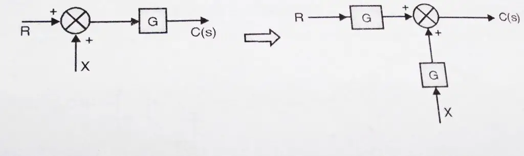
Rule 5:  Shifting of a Summing Point before a block

When we shift the summing point before a block, we need to do the transformation in order to achieve the same result. Please refer to the diagram below :

C(s) = GR(s) + X

After shifting the summing point, we will get

C(s) = [R +(X/G) ] G = GR + X which is same as output in the first case.

Hence to shift a summing point before a block, we need o to add another block of transfer function ‘1/G’ before the summing point as shown in figure. 

Rule 6: Shifting of the Summing Point after a block

When we generally shift the summing point after any block, we required to do the transformation to attain the same (required) result. Please refer the below diagram . 

 

C(s) = (R + X)G

After shifting the summing point, we will get

C(s) = (R +X) G = GR + XG which is same as output in the first case.

Hence to shift a summing point before a block, we need to add another block having the same transfer function  at  the summing point as shown in fig

Rule 7: Shifting of Take-off point after a block

Here we want to shift the take – off point after a block, as shown in the diagram

 

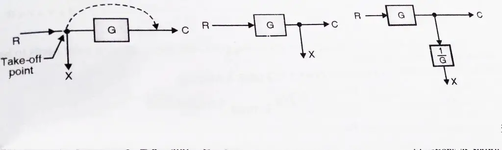
Here we have X = R and C = RG (initially)

In order to achieve this, we need to add a block of transfer function ‘1/G’ in series with signal taking off from that point.

Rule 8 : Shifting of Take-off point before a block

Here we want to shift the take – off point before a block, as shown in the diagram

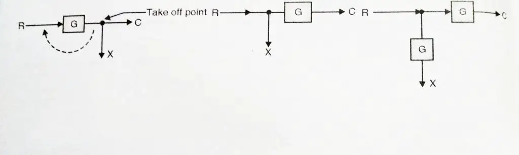
Here we have X = R and C = RG (initially)

In order to achieve this, we need to add a block of transfer function ‘G’ in series with X signal taking off from that point.

Rule 9 : Shifting a Take-off point after a Summing Point

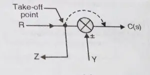
can be transformed to (refer both the diagrams)

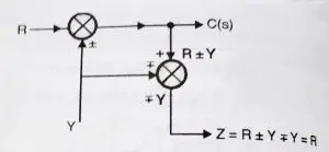
Before shifting take-off point, initially, we have:

C(s)=R±Y

and Z = R ± Y (initially)

Hence if we want to shift a take-off point after a summing point, one more summing point needs to be added in series with take-off point.

Rule 10: Shifting a take-off point before a summing point

Suppose if we want to shift take-off point before a summing point, then initially we have

C(s)=R±Y

and Z = R ± Y (initially)

 

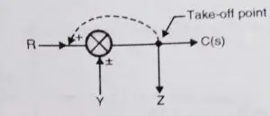
this can be transformed to (refer both the diagrams)

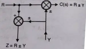
In order to satisfy this condition, we need to add a summing point in series with the take-off point.

Note:

1. Rules 9 and 10 are critical rules, their usage should be avoided as much as possible(i.e if there is no other options present then only we should use them).

2. Always try to shift take-off points towards right and summing points towards left

If there are multiple inputs present, then we have to use the superposition theorem(which means we have to consider one input at a time and find out the output considering all other inputs to be zero and finally taking the summation of all the output thus obtained).

Advantages Of Block Reduction Technique !!

Though there are many other methods present to solve any complex block arrangements (seen in the later posts) , this block reduction rules often come handy due to the following reasons :

1. With these blocks reducing shortcuts, you can easily break a complex LTI  (linear time-invariant) control system into simple blocks and then reduce it to get the required output easily .

2. You can individually visualize the various components of any given complicated control system easily , which can be helpful while analyzing any issue or to study separate parts of any LTI system .

Finally, we reach the end of this wonderful(time-consuming :-p) post. Block reduction technique is one of the many (other methods discussed in later posts) methods available to deal with complex block diagrams in the Control System.

Hope you really liked this post , let me know your thoughts in the comments section. Stay tuned for the next post in this series (with solved examples for block diagram reduction related to this topic). 

Read More :

1. Complete analysis of Bode Plot

2. A to Z about the Root Locus in Control System

3. Complete overview of the Polar Plot

4. Details about the Nyquist Plot