Control System – Transfer Functions

Howdy, fellas!!

I hope you already acquaint yourself with the Control System subject overview (from my previous posts). So let’s not waste our time further and get started with the basics of this subject(i.e the Transfer Function overview which is the basic building block of any control system) .

In Control systems, we mainly deals with mathematical models  and their analysis. So we should first understand what mathematical modelling is ??

Modelling something is a way to express their systems in math terms allowing to utilize the physics concepts on it. We truly need some representation of our plant in writing, since it is very costly to be able to always check and experiment different inputs and parameters repeatedly for just about any process that is exactly same.

A model that is mathematical provides the straightforward, demonstrative and appreciable interpolation and extrapolation of this process we are concerned of. This model further assist us to design the controllers and control system that is optimal.

In Control Systems, models are referred to as systems. A system is represented as a block consists of atleast one input and output signal. Further, the input will be referred as ‘excitation’ and output as ‘response’.

So what exactly the transfer function is ?

For almost any control system, there fundamentally exists a reference input that is referred to as the main cause or excitation which generally runs via a series of transfer processes known as the transfer function and creates an effect causing the response reaction. Therefore the reason and the impact relationship between an input and output is therefore linked to one another through the transfer function.

Definition: A transfer function in any control system is defined as the ratio of Laplace transform of the output to that of the Laplace transform of given input function assuming all the initial conditions to be zero.

What is the use of the Laplace transforms?​

Transfer function of any system is basically used for the mathematical evaluation of any system (consists of differential equations). Laplace is the easiest form to resolve any differential equation . In most of the cases , the input and the output of any given system may not be in same category.

For instance, a motor generally converts the electrical power into mechanical form of energy. It is furthermore important to express the output and input in the form of same quantity mainly for the feasibility of the mathematical analysis. Hence we generally use the Laplace transforms for the transformations (conversions) of all kinds of signals to a simple common form.

What does it mean by initial conditions are zero?

We take the initial condition to be zero in order to make RHS of transfer function independent of the input. The transfer function method is mainly valid for the linear time invariant (LTI) systems. All the electrical control systems generally consists of the  R, C or L elements or the mixture of any of theses elements .

These parameters are linear time invariant (LTI) which means that their values do not change with regards to time. Since these parameters are independent of the variations of time parameter, we thus must proceed with the approach that is same for any control system.

Hence we consider (assume) all the initial conditions to be zero.( this can be a demerit of utilizing a transfer system. But this might be taken well cared in state space analysis).

Method of finding transfer function:

• We need to first find separate equations for input and output in any given physical system
• Now we shall take the Laplace transform of the system equations, thereby assuming the initial conditions as zero.
• Finally we have to take ratio of the Laplace transforms of output and input.

 

Poles and Zeroes of a transfer function:

In layman terms, we can say that the Poles and Zeros of any transfer function are simply the frequencies for which the values of the numerator and denominator of  the transfer function becomes zero .

Why Poles and Zeros important?

It defines and helps us to determine the stability of the system, which is very critical (this aspect we will learn in my later posts)

Poles: These are the values of Laplace transform variable, which makes the transfer function to become infinite. Poles we can find out by equating the denominator of any transfer function to zero.

Zeroes: These are the values of Laplace transform variable, which makes the transfer function to become zero. Zeros we can find out by equating the numerator of the transfer function to zero.

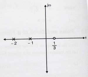
In the Laplace plane(s-plane) we have two axis(s= σ+jω) i.e imaginary axis(jω) and   real axis (σ). Poles are represented by “x” and zeros are represented as “o” on s plane.

If the transfer function is given as :

To find poles, we will equate denominator to zero and for zeros, we will equate numerator to zero.

on equating we get,

2 poles i.e s = -2,-1  and  one zero i.e s = 1/3  (as shown below)

 

Some important points to be noted regarding Transfer Function

 

1. The concept of transfer function is only defined for LTI systems.
2. Stability can be determined from the characteristics equation (discussed in later post)

 

Proper and improper Transfer Functions

If a transfer function has more poles than zeros (i.e order of denominator is more than order of numerator), then it is proper transfer function

And if number of zeros is more than number of poles(order of numerator more than order of denominator), then it is called improper transfer function.

Mostly we get to deal with proper transfer function, as the integrator (proper transfer function) used to reduce the amplitude of noise signals and thus surpasses the higher frequency noise. whereas the differentiator( improper transfer function) enhances the noise signals.

 

Advantages of Transfer function:

 

• From this we will get the poles and zeros, and hence we can infer the response of the system.
• The integral and differential equations can be converted to simple algebraic equation.
• This is a mathematical model that gives the gain of the given block/system.

 

Disadvantages of Transfer function:

 

• It does not take into account the initial conditions.
• Only valid for linear time invariant systems

 

Analogous Systems:

 

If we further analyse the equations (this will be discussed in detail in my later post) for mechanical translational or rotational systems with electric systems, it can be found that they are of similar forms.(I am directly giving the analogy, for the equations you can refer any standard book of Control System)

 

Force-Voltage Analogy:

 

Mechanical translational System	Mechanical rotational System	Eletrical System
Mass M	Moment of inertia – J	Inductance L
Force F	Torque – T	Voltage – V
Viscous friction Coefficient f	viscous friction coefficient –  f	Resistance R
Spring stiffness k	Tortional spring Stiffness k	Reciprocal of capacitance  1/C
Velocity  v	Angular velocity- ω	Current i
Displacement x	Angular displacement-θ	Charge q

 

Force – Current analogy:

 

Mechanical translational System	Mechanical rotational System	Eletrical System
Mass M	Moment of inertia – J	Capacitance  C
Force F	Torque – T	Current   i
Viscous friction Coefficient    f	viscous friction coefficient –  f	Reciprocal of Resistance 1/R
Spring stiffness k	Tortional spring Stiffness k	Reciprocal of inductance  1/C
Displacement x	Angular displacement-θ	Magnetic Flux Linkage φ
Velocity  v	Angular velocity- ω	Voltage V

 

From the above, it is much evident that all the three systems are analogous to each other and equations of one system can be converted into other.