Control System – State Space Model

July 29, 2018June 17, 2020 Techie Aric 0 Comments

In my previous post we have seen that the state space model of a Linear Time-Invariant (LTI) system is represented as,

$\dot { x }$ (t) = A x(t) + B x(t) ,

y(t) = Cx(t) + D u(t)

Now we have a different representation of state model:

Forming state model by physical variables
Forming state model by phase variables
Canonical state variables

Forming state models by physical variables:

We now take one simple example to illustrate this:

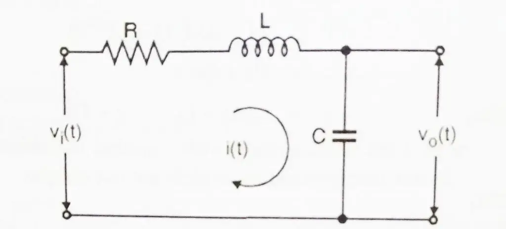
We need to obtain state model of the given RLC circuit

Control System - State Space Model

From the above circuit diagram, we can see that there are two storage elements, i.e capacitor and inductance . Hence two state variables that we can choose are

Current passing through the inductor
Voltage across capacitor

The input is represented as u(t)

Here u(t) = $v_i$ (t) ,

The state variables are $x_1$

(t) = i(t) ; $x_2$ (t) = $v_0$

(t) …….. (1.1)

We now apply KVL , $v_i$ (t) = Ri(t) + L $\frac{d}{dt}$ i(t) + $v_0$ (t) ………. (1.2)

We write equation (1.2) in terms of $\frac{d}{dt}$ i(t)

Hence, $\frac{d}{dt}$ i(t) = $\frac{1}{L}v_i$ (t) – $\frac{R}{L}$ i(t) – $\frac{1}{L}v_0$ (t) …….. (1.3)

$i_1$ (t) is the state variable $x_1$ (t)

$\frac{d}{dt}i_1$ (t) = $\frac{d}{dt}x_1$ (t) = $\dot{x}$ (t)

Similarly $v_i$ (t) is the input, $v_i$ (t) = u(t) ,

$v_0$ (t) is the state variable $x_2$ (t) ,

Using these in equation (1.3) we get,

$\dot{x_1}$ (t) = $\frac{1}{L}$ u(t) – $\frac{R}{L}x_1$ (t) – $\frac{1}{L}x_2$ (t) ……. (1.4)

We know that $v_0$ (t) is the voltage across the capacitor

$v_0$ (t) = $\frac{1}{C}\int { i(t)dt }$ ,

Differentiating both sides, we get

$\frac{d}{dt}v_0$ (t) = $\frac{1}{C}$ i(t)

We now put $v_0$ (t) = $x_2$ (t) and i(t) = $x_1$ (t) ,

$\dot{x_2}$ (t) = $\frac{1}{C}x_1$ (t) …………. (1.5)

Equation (1.4) and equation (1.5) give us the state equation

$\begin{bmatrix} \dot { { X }_{ 1 } } (t) \\ \dot { { X }_{ 2 }(t) } \end{bmatrix}$ = $\begin{bmatrix} -\frac { R }{ L } & -\frac { 1 }{ L } \\ \frac { 1 }{ C } & 0 \end{bmatrix}\begin{bmatrix} { x }_{ 1 }(t) \\ { x }_{ 2 }(t) \end{bmatrix}$ + $\begin{bmatrix} \frac { 1 }{ L } \\ 0 \end{bmatrix}$ u(t) ,

This is of the form $\dot{X}$ = A x(t) + Bu(t)

For the output we have,

y(t) = $v_0$ (t) = $x_2$ (t) y(t) = $\begin{bmatrix} 0 & 1 \end{bmatrix}\begin{bmatrix} { x }_{ 1 }(t) \\ { x }_{ 2 }(t) \end{bmatrix}$ + $\begin{bmatrix} 0 \end{bmatrix}$ u(t) ,

This is of the form Y = Cx(t) + D u(t)

Now we will see some important properties of state transition matrix:

The state transition matrix gives idea about the progress of state fro x(0) , It gives the free response of the system.

Φ(0) = $e^{A0}$ = I ,
Φ(t) = $e^{At}$ = ${ \begin{bmatrix} \Phi (-t) \end{bmatrix} }^{ -1 }$ ,
${ \begin{bmatrix} \Phi (t) \end{bmatrix} }^{ n }$ = Φ(nt) ,
Φ( $t_2-t_1$ ) Φ( $t_1-t_0$ ) = Φ( $t_2-t_0$ ) ,

How to obtain Transfer function from State Variable Model and Vise versa:

We already know that apart from internal behaviour , the state variable model yields the input output behaviour as well.Hence we can convert the state variable to its transfer function form and vice versa.

Now consider a SISO case, whose state and output equations are given as :

$\dot{x}(t)$ = Ax(t) + Br(t) …… (1.6)

y(t) = Cx(t) + Dr(t) …….(1.7)

To obtain transfer function, we take its Laplace transformations.

Hence, sX(s) – s( $t_0$ ) = AX(s) + BR(s)

Here x( $t_0$ ) indicates initial condition.

Now assuming zero initial conditions, i.e x( $t_0$ ) = 0 ,

sX(s) = AX(s) + BR(s)

Then , (sI-A)X(s) = BR(s) ,

Now, X(s) = ${(sI-A)}^{-1}BR(s)$ …… (1.10)

Taking Laplace Transform of equ (1.7) , Y(s) = CX(s) + DR(s) , ……. (1.11)

Putting equ (1.10) in equ (1.11) we get,

Now, Y(s) = C ${[sI-A]}^{-1}]$ BR(s) + DR(s) ,

Hence , C $[{(sI-A)}^{-1}B + D]$ R(s) ,

Hence we get transfer function T(s) = $\frac{Y(s)}{R(s)}$ = C $[{(sI-A)}^{-1}B + D]$ ,

Concept of controllability and observability :

Controllability:

In the control system, there are many systems that is required to be controlled. The concept of controllability refers to the capability of any controller in order to arbitrarily modify the functionality of the system plant. Controllability implies the ability to change the state by input.

A process is said to be controllable if for the system it is possible to transfer the system from the initial state i.e x( $t_0$ ) to some other desired state i.e x( $t_t$ ) in a specified time.

Observability :

We have seen that the state variable of a system , x , represents the internal working of the system. This also needs to be observed along with the output and the input .This term describes if any internal state variables of any particular system can be externally measured.Thus a process is said to be observable if every state x( $t_0$ ) can be easily determined by the measurements of the output y(t) over a specific time duration .

Techie Aric

Aric is a tech enthusiast , who love to write about the tech related products and ‘How To’ blogs . IT Engineer by profession , right now working in the Automation field in a Software product company . The other hobbies includes singing , trekking and writing blogs .

Spread the Wisdom !!

Techie Aric

Aric is a tech enthusiast , who love to write about the tech related products and 'How To' blogs . IT Engineer by profession , right now working in the Automation field in a Software product company . The other hobbies includes singing , trekking and writing blogs .

Techie Aric

You May Also Like

Leave a Reply Cancel reply