Graphing Inequalities – Steps To Solve Inequalities Graph In Two Variables With Examples !!

Graphing inequalities equation is another way of solving any given inequality quickly. In the graphical solution of inequations, the first step is to plot the graph of the given inequality. We already know the steps to find and solve any given inequality. Now in this post, we’ll see the different steps involved in solving inequalities graphically.

If a ,b ,c are real numbers, then the equation ax + by + c = 0 is called a linear equation in two variables ‘x’ and ‘y’ whereas the inequations :

ax + by < c  , ax +by > c , ax + by ≤ c ,  ax + by ≥ c    ;

are called linear inequalities in two variables ‘x’ and ‘y’. Now let’s see the exact steps you need to follow to solve any inequalities graphically.

Steps For Graphing Inequalities On Number Line In Two Variables ?

In order to find the solution set of any given inequalities graphically, we have to follow the following steps:

• Convert the given inequality, say ax + by ≤ c , into the normal equation ax + by = c , which represents a straight line on the xy plane.
• Now put y = 0 in the equation obtained in the above step to get the point where the line meets with the x-axis. Then put x =0 , to obtain a point where the line meets the y-axis respectively .
• Join the points obtained in step second to obtain the graph of the line obtained from given inequality.
• Now choose a point i.e (0,0) not lying on this line. Substitute its coordinates in the given inequality. If the inequation is satisfied then shade the portion of the graph which contains the chosen point (i.e. origin) otherwise shade the portion which doesn’t contain the chosen point that is (0,0).
• Finally, the shaded region in the above step represents the given required solution set for the given inequalities equation graphically .

Note : in case of the inequalities that is ax + by ≤ c and ax + by ≥ c , all the points on the line ax + by = c are also part of the shaded region (part of the solution set). While in the case of inequalities ax + by < c and ax + by > c , all the points on the line ax + by = c ,  will not be in the shaded region (part of the solution set).

The graph of any linear equation basically represents a straight line dividing the complete xy-plane into two parts. The complete xy-plane will be divided into two parts represented by ax + by ≤ c and ax + by ≥ c . These two parts are known as the closed half spaces .

The complete xy-plane will be divided into two parts represented by ax + by < c and ax + by > c . These two parts are known as the open half spaces .

These half-spaces on the xy-plane typically represent the complete solution set of any given linear inequalities graphically. Look at the below graph for a simple linear equation for reference. 

Steps To Solve Inequalities Graph In Two Variables !!

As seen above , we need to just follow the steps respectively to find the final solution set of any inequalities graphically . Now it’s time to solve some inequations examples using the above-mentioned equations, let’s solve the inequalities graph now :

1. Let’s find the solution set for the given inequality below using graph 

        2x – y ≥ 1 

According to the first step, we need to convert this inequality equation into a simple equation with the equality sign first.

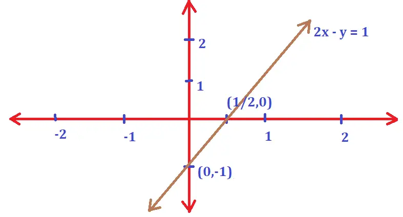
Hence after reducing the given inequation, we will get the linear equation as :   2x – y = 1 .

Now as per the next step, we need to plot the graph of the given equation. This can be done by putting the values of ‘x’ and ‘y’ as ‘0’ in the above equation to obtain the points where the line meets the Y and X axis respectively.

On putting  ‘x = 0‘ we get the value of ‘y’ as -1. Similarly, on putting ‘y = 0‘ we get the value of x as ‘1/2’.

This means that the given line meets the x and y axes at A(1/2 , 0) and B (0 , -1) respectively .

Now to obtain the graph of the given equation, we need to join these two points in the xy plane. On joining the points we will get a straight line dividing the complete xy-plane into two regions.

As it is evident from the graph, we have the origin that is (0,0) is present in one of the regions formed by plotting the graph of the given equation.

Now if we put the values of origin (0,0) in the given inequality that is 2x – y ≥ 1 . Then clearly the values will not satisfy the given inequation.

So we need to take the other region as the final solution set for the given inequality. So the region not containing the origin is represented by the given inequality and it can be shown in the graph format as given below.

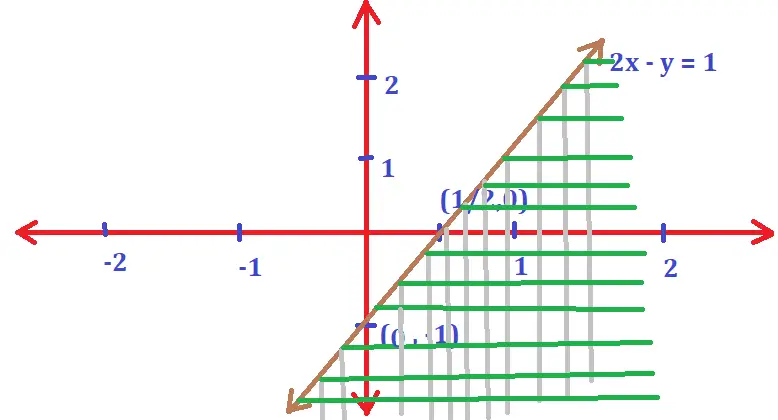
Since we also have equality sign in-between the inequality sign i.e. ‘≥’  in the given equation, thus we also need to include all the points present on the line as the solution set for the given inequality from the graph .

Now let’s solve a given inequality including the absolute values graphically.

How To Solve Inequalities Graphically For Absolute Values In Two Variables ?

For any absolute values inequality, we need to follow similar steps as given above. Always remember that an absolute value includes both the positive and negative values respectively. Let’s solve some examples to make this concept clear.

Let say the given inequality is :  |x – y|  ≥  1 

We have |x – y|  ≥  1  as the given inequality to be solved graphically, also from the definitions of absolute values we can write the above inequation as below :

x – y  ≥  1,   and 

-(x – y)  ≥  1

Now multiplying the second inequation with ‘-1’ on both the sides respectively, the sign of the inequality changes as :

(x – y)  ≤  -1

Now we have to plot the graph of two equations respectively i.e. ‘x – y – 1 ≥ 0‘  and  ‘x – y + 1 ≤ 0‘ . Now we need to plot the graph for each of these lines separately and then need to merge the solution set of both to get the final solution from graph .

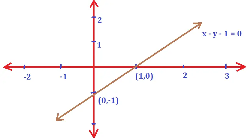
For the first equation i.e   x – y – 1 = 0 , on putting x = 0 we get y = -1 . And also on putting y = 0 , we get x = 1 . So the points where the line cuts the x and y axes respectively will be A(1,0) and B(0,-1)

For the second equation i.e   x – y + 1 = 0 , on putting x = 0 we get y = 1 . And also on putting y = 0 , we get x = -1 . So the points where the line cuts the x and y axes respectively will be A(-1,0) and B(0,1)

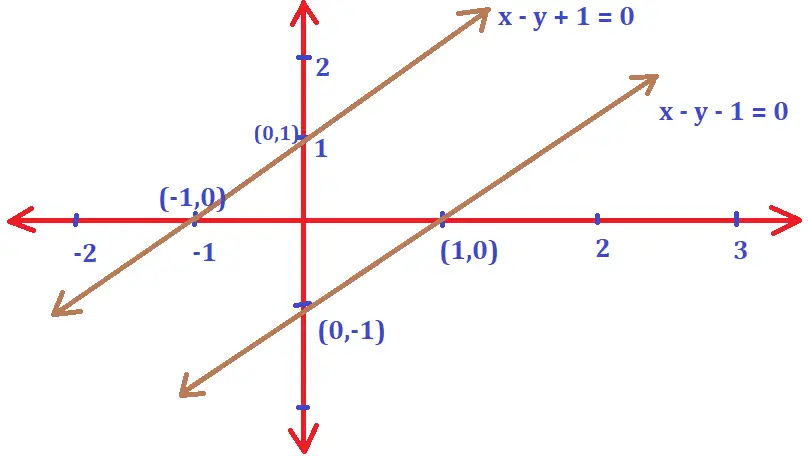
Now as the final step, we again put the point (0,0) in the above-given inequations to find the solution set for the given inequalities. The final solution set will be the union of both the regions represented by x – y – 1 ≥ 0‘  and  ‘x – y + 1 ≤ 0 .

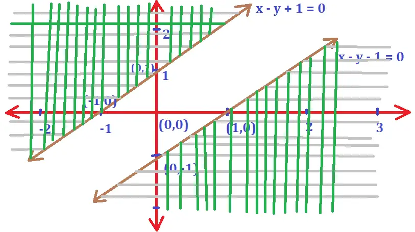
Hence on putting the point of origin i.e. (0,0) in both the inequalities i.e. ‘x – y – 1 ≥ 0‘  and  ‘x – y + 1 ≤ 0′  . Clearly it doesn’t satisfy the given inequalities. Hence we need to take the other region that is the region that doesn’t contain origin as the solution for both the inequalities.

Graphing Inequalities In Two Variables For Set Of Two Or More Inequations !!

In this section, we’ll understand the technique of finding the solution set of two simultaneous inequalities graphically. Basically in this type of inequalities, different constraints will be given, and based upon the given conditions we need to find the regions satisfying the given inequality in the xy plane .

Mostly the solution set of simultaneous linear inequations may be an empty set or maybe the region bounded by the straight-line boundaries.

Let’s solve one example related to the simultaneous inequalities graph.

Let say the given inequalities as :      3x + 4y ≤ 12 ,  4x + 3y ≤ 12  ,   x ≥ 0  ,   y  ≥  0    ;

The first step is to convert the given inequalities into normal equations, then the inequalities will be reduced to the normal equations as

3x + 4y = 12 ,  4x + 3y = 12  ,   x = 0  ,   y  =  0     ;

Let us now solve each inequality separately .

Region represented by the inequality 3x + 4y ≤ 12  :

Once we reduce this inequality into a normal equation , then the given equation will be 3x + 4y = 12 . This is a straight line . Now we need to find the points on the x and y-axis where the given line cuts the respective axes.

On putting x = 0 , we will get the point on the y-axis, and similarly on putting y = 0  , then we’ll get the point on the x axis . The two points will be A(4,0) and B(0,3) .

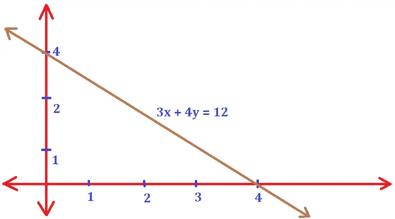
Now we need to find the solution set of this given inequality by putting the origin (0,0) on the equation as we did earlier.

On putting the point (0,0) , it will satisfy the given inequality i.e. 3x + 4y ≤ 12. Hence the portion containing the origin represents the solution set of the given inequation i.e. 3x + 4y ≤ 12 .

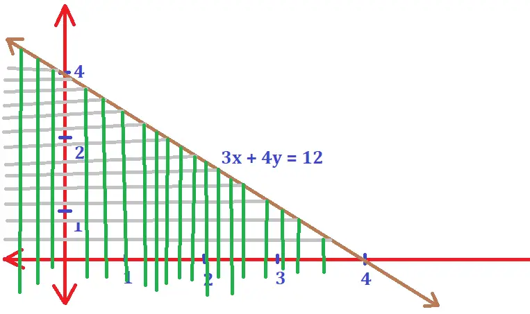
This can be represented in the graph as above .

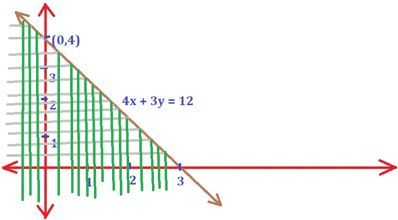
Region represented by 4x + 3y ≤ 12 :

Once we reduce this inequality into a normal equation , then the given equation will be 4x + 3y = 12 . This is indeed a straight line . Now we need to find the points on the x and y-axis where the given line cuts the respective axes.

On putting x = 0 , we will get the point on the y-axis, and similarly, on putting y = 0, we will get the point on the x-axis . The two points will be A(3,0) and B(0,4) .

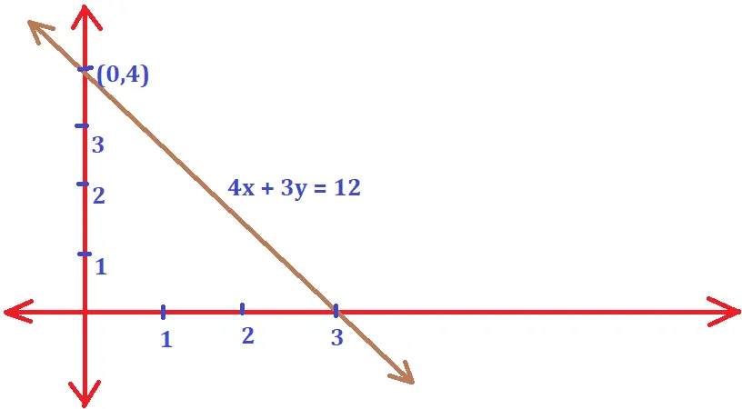
Now we need to find the solution set of this given inequality by putting the origin (0,0) on the equation as we did earlier.

On putting the point (0,0) , it will satisfy the given inequality i.e. 4x + 3y ≤ 12. Hence the portion containing the origin represents the solution set of the given inequation i.e. 4x + 3y ≤ 12 .

Region represented by     x  ≥  0  and   y  ≥ 0   ;

Clearly x ≥ 0 and y  ≥ 0 represents the first quadrant of the cartesian plane. Now for the final resultant solution set of the given inequalities, we need to take the common region represented by all the above-given inequalities . 

Note: In order to derive the common region, we need to apply the rule of the intersection of figures . Here the common region satisfying all the given set of constraints will be considered as the final solution set on graphing inequalities.

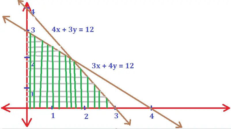
Hence the shaded region represents the solution set of the given set of linear inequalities .

Hope you really liked this post regarding the steps to solve inequalities using graph . Let me know in the comments, if you have any doubts . Stay tuned for more interesting stuff in this series .