Control System – State Space Analysis

July 26, 2018June 17, 2020 Techie Aric 0 Comments

In this post we will see the state variable model of a system. As compared to the transfer function approach , the state variable approach gives us the timely behaviour of internal variables of a model. This can be used to analyze both time-invariant and nonlinear systems as well.

Before we further proceed we should understand the difference between state-space analysis and transfer function.

In transfer function, it is assumed that the initial conditions of the system are zero(in many practical examples, the initial conditions are not equal to zero).

While making a state-space analysis , no such assumptions are necessary. It will be applicable even if the initial conditions are not zero. The state variable description is more general than the transfer function .

Concept of State , State variables, and State model :

What is meant by state?

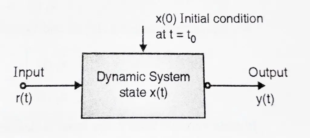
It can be defined as a minimal set of variables(called as state variables) such that the knowledge of these variables at $t = t_0$ together with the knowledge of inputs for $t\ge0$ completely determines the behavior of the system for $t>t_0$ .

Control System - State Space Analysis

State variables:

The smallest set of variables determines the state of dynamic system. For ‘n’ variables $x_1(t)$ , $x_2(t)$

, …… $x_n(t)$ are needed to completely describe the behavior of a dynamic system, together with initial state and inputs, then these set of ‘n’ variables are called asset of state variables. The state vector x(t) is the vector sum of all the state variables.

State vector :

If ‘n’ state variables are needed to completely describe the behavior of a given system, then these ‘n’ state variables can be considered to be n components of a vector x(t). Such a vector is called a state vector . It uniquely determines the system state x(t) for any time t $\ge$ $t_0$ .

State space:

The n dimensional space whose co-ordinate axis consists of the $x_1$ axis , $x_2$ axis ….. $x_n$ axis is called a state space . Any state can be represented by a point in the state space. Consider a mechanical system , mass M is acted upon by a force F(t).(in this case we assume zero friction)

M = mass of body F(t) = force

P(t) = displacement v(t) = velocity

Let the state variables be

Displacement p(t)
Velocity v(t)

Hence, $x_1(t)$ = p(t) and $x_2(t)$ = v(t) ,

From physics we know,

F = M $\times$ a

F = M $\times$ $\frac{dv(t)}{dt}$ ,

Hence $\frac{dv(t)}{dt}$ = $\frac{F(t)}{M}$ ,

This we can now write in terms of state variable as:

$\dot { { X }_{ 2 } }$ = $\frac{F(t)}{M}$ ……. (1.1)

Also $\dot { { X }_{ 1 } }$ = $x_2(t)$ ………… (1.2)

We now represent above two equations in matrix form as :

$\begin{bmatrix} \dot { { X }_{ 1 }(t) } \\ \dot { { X }_{ 2 }(t) } \end{bmatrix}$ = $\begin{bmatrix} 0 & 1 \\ 0 & 0 \end{bmatrix}\begin{bmatrix} { x }_{ 1 }t \\ { x }_{ 2 }t \end{bmatrix}$ + $\begin{bmatrix} 0 \\ \frac { 1 }{ M } \end{bmatrix}$ F(t) ,

In state variable theory, the input is defined as r(t), hence

F(t) = r(t) ,

Above equation will be modified to give

Now if the desired output is velocity then,

Y(t) = v(t)

In matrix form we get,

Y = $\begin{bmatrix} 0 & 1 \end{bmatrix}\begin{bmatrix} { x }_{ 1 }(t) \\ { x }_{ 2 }(t) \end{bmatrix}$ ………. (1.4)

Equations 1.3 and 1.4 are the state equations and the output equation.They can be written in the form as :

Ẋ = Ax + r = state equation

Y = $c^{'}$ x = output equation

Where, A = matrix x = vector

$c^{'}$ = vector transpose and y = scalar value

State variable representation of control system:

State model:

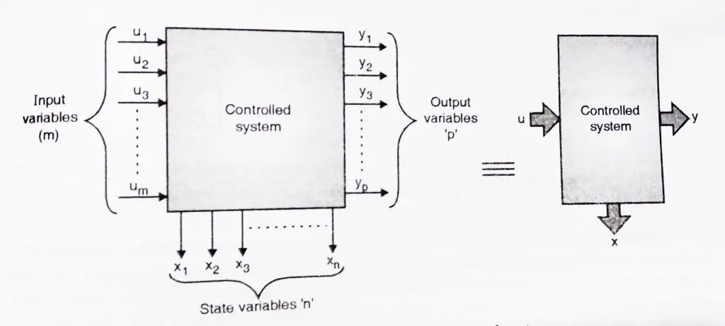
Consider a system which is multiple input multiple output(MIMO)

Let, number of inputs = m

Number of state variables = n

Number of outputs = p

Control System - State Space Analysis

The n state variables are given by n first order differential equations as follows:

$\frac{dx_1}{dt}$ = $\dot { { x }_{ 1 } }$ = $f_1$ ( $x_1$ , $x_2$ ,……, $x_n$ ; $u_1$ , $u_2$ , …. $u_m$ )

$\frac{dx_2}{dt}$ = $\dot { { x }_{ 2 } }$ = $f_2$ ( $x_1$ , $x_2$ ,……, $x_n$ ; $u_1$ , $u_2$ , …. $u_m$ )

$\frac{dx_n}{dt}$ = $\dot { { x }_{ 3 } }$ = $f_n$ ( $x_1$ , $x_2$ ,……, $x_n$ ; $u_1$ , $u_2$ , …. $u_m$ ) ……………. (1.5)

The n differential equation can be written in a vector notation as ,

$\dot { { x(t) } }$ = f(x(t) , u(t)) ……………… (1.6)

for a time varying system, t also becomes a parameter

$\dot { { x(t) } }$ = f(x(t) , u(t), t) ……………….(1.7)

similarly the relationship between p outputs can be given as ,

$y_1$ = $g_1$ ( $x_1$ , $x_2$ ,……, $x_n$ ; $u_1$ , $u_2$ , …. $u_m$ ) ,

$y_2$ = $g_2$ ( $x_1$ , $x_2$ ,……, $x_n$ ; $u_1$ , $u_2$ , …. $u_m$ ) ,

Hence in general……

$y_p$ = $g_p$ ( $x_1$ , $x_2$ ,……, $x_n$ ; $u_1$ , $u_2$ , …. $u_m$ ) ……………….. (1.8)

The equations can be written in vector notation as ,

y(t) = g( x(t) , u(t)) …………………………. (1.9)

for time varying case,

y(t) = g( x(t) , u(t), t) …………………………. (1.10)

The vector notation being

State vector x(t) = $\begin{bmatrix} { x }_{ 1 }(t) \\ \vdots \\ { x }_{ n }(t) \end{bmatrix}$ Input vector u(t) = $\begin{bmatrix} { u }_{ 1 }(t) \\ \vdots \\ { u }_{ n }(t) \end{bmatrix}$ ,

Output vector y(t) = $\begin{bmatrix} { y }_{ 1 }(t) \\ \vdots \\ { y }_{ n }(t) \end{bmatrix}$

Equation 1.5 is an expanded form of equation 1.6, and is called State equation for a linear time invariant case and equation 1.7 is the state equation for a linear time varying case. The state variables $x_1$ , $x_2$ , ……. $x_n$ from the n dimension space is called State space . The state vector ‘x’ for a particular value of $x_1$ , $x_2$ , ……. $x_n$ forms a point called state point in this state space. The trajectory traced by a state point from t = $t_0$ to t = $t_1$ is called state trajectory.

Also equation 1.8 is an expanded form of the equation and is called output equation for a linear time-invariant case and equation 1.10 is for the linear time-varying case. The state and output equations together constitute the state model of a system.

State Model of Linear Systems :

For a special case of linear time invariant systems equation 1.5 becomes,

$\dot { { x }_{ 1 } }$ = ${ a }_{ 11 }{ x }_{ 1 }+{ a }_{ 12 }{ x }_{ 2 }+\dots \dots { a }_{ 1n }{ x }_{ n }+{ b }_{ 11 }{ u }_{ 1 }+{ b }_{ 12 }{ u }_{ 2 }+\dots\dots{ b }_{ 1m }{ u }_{ m }$ ,

$\dot { { x }_{ 2 } }$ = ${ a }_{ 21 }{ x }_{ 1 }+{ a }_{ 22 }{ x }_{ 2 }+\dots \dots { a }_{ 2n }{ x }_{ n }+{ b }_{ 21 }{ u }_{ 1 }+{ b }_{ 22 }{ u }_{ 2 }+\dots\dots{ b }_{ 2m }{ u }_{ m }$ ,

Thus,

$\dot { { x }_{ n } }$ = ${ a }_{ n1 }{ x }_{ 1 }+{ a }_{ n2 }{ x }_{ 2 }+\dots \dots { a }_{ nn }{ x }_{ n }+{ b }_{ n1 }{ u }_{ 1 }+{ b }_{ n2 }{ u }_{ 2 }+\dots\dots{ b }_{ nm }{ u }_{ m }$ ,

$\begin{bmatrix} \dot { { X }_{ 1 } } \\ \vdots \\ \dot { { X }_{ n } } \end{bmatrix}$ = $\begin{bmatrix} { a }_{ 11 } & \dots & { a }_{ 1n } \\ \vdots & \vdots & \vdots \\ { a }_{ n1 } & \cdots & { a }_{ nn } \end{bmatrix}\begin{bmatrix} { x }_{ 1 }(t) \\ \vdots \\ { x }_{ n }(t) \end{bmatrix}\quad+\quad\begin{bmatrix} { b }_{ 11 } & \dots & { b }_{ 1n } \\ \vdots & \vdots & \vdots \\ { b }_{ n1 } & \cdots & { b }_{ nn } \end{bmatrix}\begin{bmatrix} { u }_{ 1 }(t) \\ \vdots \\ { u }_{ n }(t) \end{bmatrix}$ ……… (1.11)

i.e $\dot { { x } }$ (t) = A x(t) + B x(t) ,

where A = $\begin{bmatrix} { a }_{ 11 } & \dots & { a }_{ 1n } \\ \vdots & \vdots & \vdots \\ { a }_{ n1 } & \cdots & { a }_{ nn } \end{bmatrix}$ = System matrix = (n x m ) matrix ,

B = $\begin{bmatrix} { b }_{ 11 } & \dots & { b }_{ 1n } \\ \vdots & \vdots & \vdots \\ { b }_{ n1 } & \cdots & { b }_{ nn } \end{bmatrix}$ = Input matrix = (n x m) matrix ,

X(t) = state vector = n $\times$ 1

U(t) = input vector = m $\times$ 1

Equation 1.11 is the state equation.

Output equation: it can be similarly derived as,

$y_1(t)$ = ${ c }_{ 11 }{ x }_{ 1 }(t)+{ c }_{ 12 }{ x }_{ 2 }(t)+\dots \dots { c }_{ 1n }{ x }_{ n }(t)+{ d }_{ 11 }{ u }_{ 1 }(t)+{ d }_{ 12 }{ u }_{ 2 }(t)+\dots\dots{ d }_{ 1m }{ u }_{ m }(t)$ ,

$y_2(t)$ = ${ c }_{ 21 }{ x }_{ 1 }(t)+{ c }_{ 22 }{ x }_{ 2 }(t)+\dots \dots { c }_{ 2n }{ x }_{ n }(t)+{ d }_{ 21 }{ u }_{ 1 }(t)+{ d }_{ 22 }{ u }_{ 2 }(t)+\dots\dots{ d }_{ 2m }{ u }_{ m }(t)$ ,

Thus,

$y_p(t)$ = ${ c }_{ p1 }{ x }_{ 1 }(t)+{ c }_{ p2 }{ x }_{ 2 }(t)+\dots \dots { c }_{ pn }{ x }_{ n }(t)+{ d }_{ p1 }{ u }_{ 1 }(t)+{ d }_{ p2 }{ u }_{ 2 }(t)+\dots\dots{ d }_{ pm }{ u }_{ m }(t)$ ,

Y(t) = Cx(t) + D u(t)

Where C = $\begin{bmatrix} { c }_{ 11 } & \dots & { c }_{ 1n } \\ \vdots & \vdots & \vdots \\ { c }_{ p1 } & \cdots & { c }_{ pn } \end{bmatrix}$ = output matrix ( p x n)

D = $\begin{bmatrix} { d }_{ 11 } & \dots & { d }_{ 1n } \\ \vdots & \vdots & \vdots \\ { d }_{ p1 } & \cdots & { d }_{ pn } \end{bmatrix}$ = Transmission matrix ( p x m ) ,

Thus state model for a linear time invariant system is ,

$\dot { { x } }$ (t) = A x(t) + B x(t)

y(t) = Cx(t) + D u(t) ………….. (1.12)

The block diagram for equation 1.12 can be shown below as

Control System - State Space Analysis

Here we end our post, in our next post we will see the state space representation by state variables. So stay tuned for our next post in this series.

Techie Aric

Aric is a tech enthusiast , who love to write about the tech related products and ‘How To’ blogs . IT Engineer by profession , right now working in the Automation field in a Software product company . The other hobbies includes singing , trekking and writing blogs .

Spread the Wisdom !!

Techie Aric

You May Also Like

Leave a Reply Cancel reply